Often we will have an image with no geographic coordinates or incorrect geographic coordinates that must be georeferenced. Because images are usually local, georeferencing is done using a projection such as UTM. You must have a georeferenced dataset to begin with, such as another image (image to image registration), a map (image to map registration), or known coordinates at multiple points on the map (say GPS coordinates). Georeferencing can be accomplished by picking pixels on the image of known coordinates, and then warping the image to fit the coordinates.
Warping can take the form of simple rotation and translation or by "rubber sheeting" using a higher-order polynomial transformation. It is best to use the simplest warping method possible. Unless you have reason to believe your image is distorted, it is best to use only rotation and translation (a first order polynomial transformation).
Image registration is accomplished in ArcMap using the Georeferencing tool.
The image you will register is an aerial photo of the campus taken in March of 1995. This photo has not be georeferenced and you will notice that it is distinctly off-nadir (taken from an angle). Create a working directory in your class space called ImageGeoRef and download the image into your new directory.
You will register the image to a Department of Transportation Plan map. Download the georeferenced map into your directory and unzip it. The data are also available in the class directory under the folder ImageGeoRef. Open ArcMap and add the DOT plan map. You should find that the coordinate system is NAD83 UTM18N. The campus is in the lower right hand corner of the map.
Add the campus_photo.tif image to your project. If you zoom to layer, you will notice that the image is nowhere near the DOT plan map. It also is very small, with an extent of only 8 by 10 meters.
Go to View...Toolbars.. to open up the Georeferencing toolbar. Make sure that the layer is set to the campus_photo.tif.
![]()
The process will be to add control points that link the pixels on the image to georeferenced pixels on the map. You will need to place X marks on both maps, so the first thing you need to do is get them close enough to work with. Zoom in on the campus area of the DOT map so that the same approximate area of the map is displayed as is covered in the campus image. Under the Georeferencing drop down menu, click "fit to display". The campus photo should be moved to be displayed in the same approximate region as the map. You will not that the DOT image covers only a portion of the image, because the quad is split across the study area, as is usually the case.
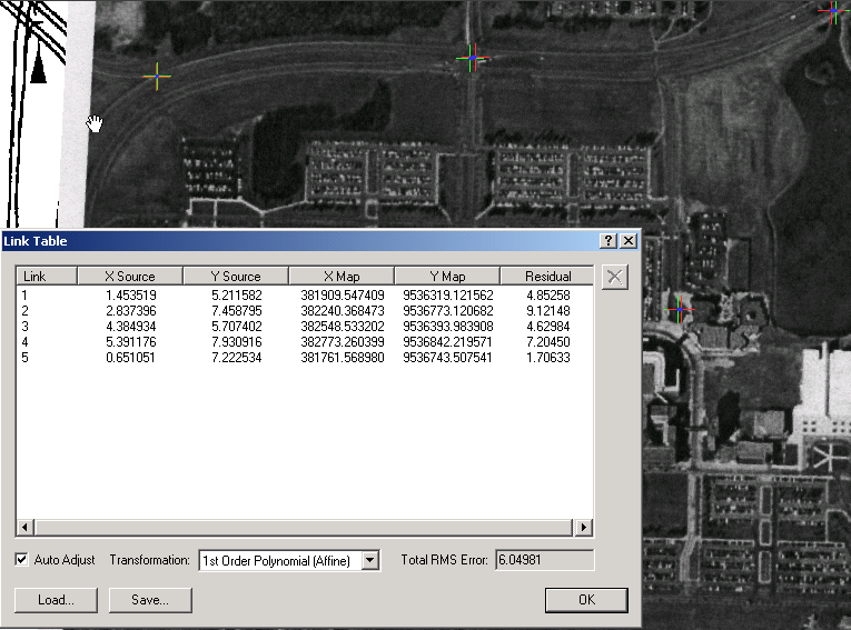
Now we can begin to add control points. Click on the control points table button ![]() . A table will be displayed that has columns for coordinates in the source (image) and the map. If you choose to Auto Adjust the image will be adjusted as you add points. This is a handy feature so leave it checked.
. A table will be displayed that has columns for coordinates in the source (image) and the map. If you choose to Auto Adjust the image will be adjusted as you add points. This is a handy feature so leave it checked.
Click on the control points ![]() button and pick a point that is easily recognizable in both the campus photo and the DOT map. Note that once you click the first control point ArcMap will draw a vector in anticipation of the next point. You can still operate zoom and view options during this time, just click the control points button again to get the cross hairs back. If you make a mistake between your first and second point, right click and choose to cancel the point.
button and pick a point that is easily recognizable in both the campus photo and the DOT map. Note that once you click the first control point ArcMap will draw a vector in anticipation of the next point. You can still operate zoom and view options during this time, just click the control points button again to get the cross hairs back. If you make a mistake between your first and second point, right click and choose to cancel the point.
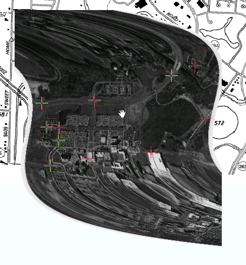
You should see the point displayed in the table. Also, the image will be moved closer to the map based upon the first one or two points you select. As you select points, ArcMap will automatically adjust the display of the image to show you how the final georeferencing will look. Note that it has not actually changed the image. You will need to do that explicitly once all your points are chosen.
After you add four points to the table a residual will be calculated for each point. This is the calculated distance between those points on the image and the map assuming the transformation indicated. If you look at the example, you will usually see that the residuals are improving as points are selected. This is because as the image is auto adjusted, it gets easy to pick reliable points. Notice that the total root mean square (RMS) error is calculated at the bottom. You objective is to get this error below 5 meters in this exercise. If you see a control point pair that has a particularly bad residual, you can delete it and try again. Remember, however, that residuals can be high because a pick is bad, or because it is a particularly important point. Try to make sure you distribute your points as much as possible throughout the image.
After you have a sufficient number of control points, you will be able to try different transformation (warping) polynomials. Try choosing a second or third order polynomial from the drop down menu at the bottom of the control points table. You will see that it "rubber" sheets the image to best fit the control points. This may or may not lower your RMS error, but you will likely find that it give very strange results at the periphery of the image where there are no control points.
Once you have entered enough points and deleted the bad points to where you have an RMS error of around 5 m, save your control points using the Save.. button at the bottom of the control points table. Then close the table and Georeferencing drop down menu choose Update Georeferencing. The points you entered will now be included in the rectification of the image. From the same drop down menu choose Rectify. The Georeferencing tool should save a seperate copy of the image.
When the tool is finished, add the georeferenced image to your project. You should see that it overlays the campus map pretty well.
Create a map of the campus, providing the title "The University at Buffalo Campus". Add all the necessary elements of a map. Also add a some call out text that points to our building, and gives the UTM and Lat-Long "Coordinates of GLY 560".
Turn the map in as a web page, and include the text table of your control points and provide the final RMS error of your image georeferencing.
THE END