You will create a simple map by "drawing" map objects on top of a base map image. This process is an alternative to the traditional approach of digitizing a map from a hardcopy, using a digitizing tablet. The advantage to digitizing on an image imported to ArcView, is that the base map can always be produced for reference or to add additional detail. Later, we will learn how to give virtually any scanned image geographical reference units, for now we will start with an image that is already georeferenced.
The example site is around Machias, New York, about 40 minutes south of here. You will transform a raster image into a vector map, by drawing in roads, streams, lakes over the image.
The USGS offers Digital Orthoquadrangle (DOQ) in a format called GeoTIFF, a georeferenced version of the popular Tagged-Image File Format (TIFF). This allows users with image rendering programs, web browsers, image processing systems, and geographic information systems to easily read and display DOQ images. If you have a program that understands GeoTIFF, the geographic reference of the image will be read in along with the image. This is an important kind of "metadata" for people who intend to use the image in conjunction with other geospatial data. This georeferencing information can be manually input to most programs that need it, but differences in reference models and input syntax can make this process time consuming and prone to error.
Geotiff DOQ's come in black and white and RGB (Red Green Blue)
color. These files can be very large, especially those with multiple
color bands. They are typically distributed as 1/4 of a quad. The
dataset you will use has be subsampled such that the original
resolution of about 1m per pixel has been reduced to about 2.2 m per
pixel. It has also been subsetted so that only a fraction of the quad
is shown. Even so, the image is about 6 MB. The original Color Geotiff
DOQ representing 1/4 of a USGS Quad was 140 MB.
Open VMWare and create a directory in your class space called
"MachiasMap"
/nsm/class/gly560/username/MachiasMap
Copy the file from the class data directory
(/nsm/class/gly560/class) called machias_geotiff.tar.gz into your
MachiasMap directory. Uncompress and untar the data.
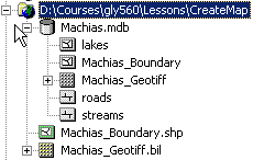
Start ArcCatalog. Create a database connection to your MachiasMap directory. In the file directory at
the left, navigate to the MachiasMap folder and the select from the top
menu File...New...Personal Geodatabase. Name the new geodatabase
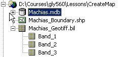
"Machias". This should see a new geodatabase in the folder
view along with your data:
You now have an empty database and some data that we want to import into this database. The data are the geotiff image and a polygon shapefile that represents the boundary of the geotiff image. This boundary file is not necessary, but will simplify the creation of new vector feature classes for this exercise.
Before we bring the geotiff into the database, lets take a look at
it. Select the machias_geotiff file and you will see its contents
in the view window to the right. Notice that the file is composed
of bands 1,2, and 3, which correspond to red, green, and blue color
components. Click on the tab marked "preview" and choose to
"build pyramids". After it is done processing, you will see the
image appear in the preview window. Now click the tab marked
"metadata". You will notice that I am too lazy to create metadata like
I should. If you click on the "Spatial" tab within metadata, you
will note that the projection of the data is UTM Zone 17N NAD27.
We will discuss the specifics of this projection type later, but for
now note that the data come with projection information which we can
use to reference any additional data.
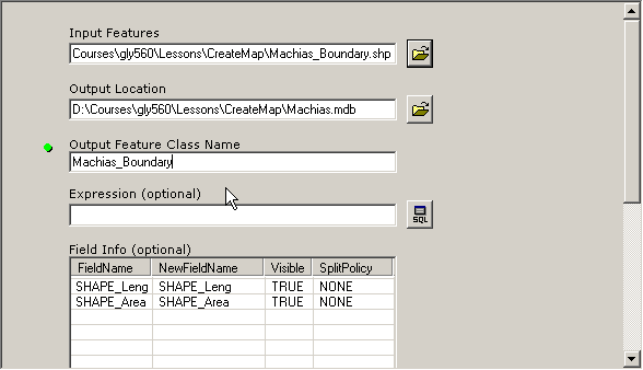
Now right-click on the database in the file index at the left and chose
Import then Feature Class (single). A new window will open that will
allow you to choose the Machias_Boundary shapefile. After you choose the file, specify Machias_Boundary again as the output class name. Click OK..
Now import the raster file Machias_Geotiff into the database using the same process. When you are done, you should have a file tree that looks like this:
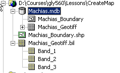
Notice that you now have copies of your data within the geodatabase, but your original files still remain in the folder.
We will create a vector file that covers the roads apparent on the
geotiff image. To do this, we have to create a new feature class
(shapefile) in our geodatabase. In ArcCatalog, select your
Machias geodatabase and pick File..New..Feature Class from the top
menu. In the wizard that opens, name the feature class "roads"
and choose next. On the next page accept the default database
configuration and choose next again. On the third page, click on
the table entry for Geometry next to SHAPE. A table for Field
Properties will be displayed below. In this table, use the
dropdown menu to the right of Geometry Type to choose line (the obvious
choice for roads).
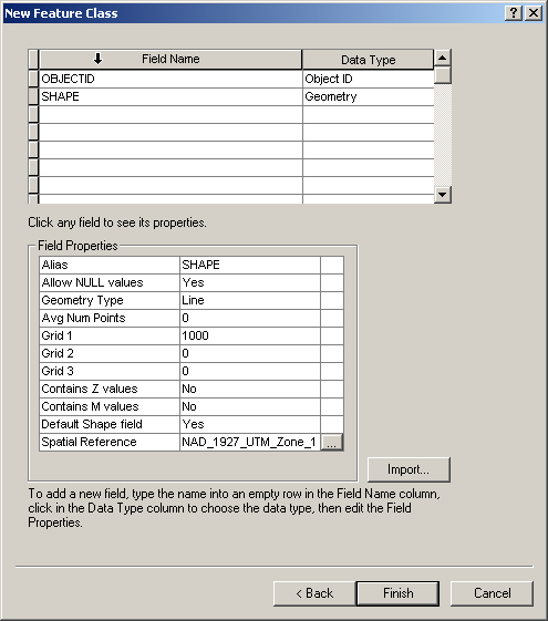
Click on the elipses to the far right of Spatial Reference. In
the dialog window that opens, choose Import. This feature allows
you to import the spatial reference from another feature class.
Double click on the database to display the Machias_Boundary feature class.
Select it and click OK. The spatial information should be
imported automatically:
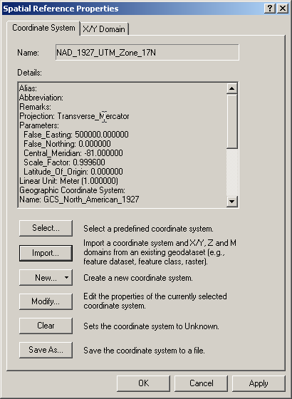
Click OK to return to the field properties. The projection
information should be displayed now in the table to the right of
Spatial Reference. Click OK and a new feature class should
be added to your geodatabase.
Repeat this process to create:
1. A line feature class named "streams"
2. A polygon feature class named "lakes".
Make sure you import the projection information from Machias_Boundary feature class. Your geodatabase should
now look like this:
Let's look at the actual files that we have stored. Look in your MachiasMap folder. You will see that the files that make up the geotiff and the shapefile are there, along with a new file and folder called Machias. This is where your data are now stored. When you store data in a geodatabase, it is all encoded into one large access file. You no longer need the original geotiff file or boundary files, so you may delete it through ArcCatalog if you wish (make sure not to delete the geodatabase!).
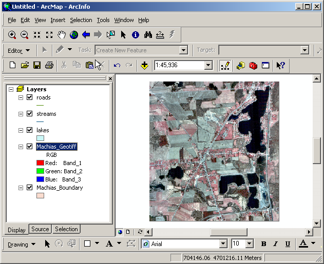
Now that we have them empty feature classes ready to go, we can start digitizing data into them. Open ArcMap by clicking on the ![]() in the menu bar. Choose to create "A New Empty Map". Using the add data button
in the menu bar. Choose to create "A New Empty Map". Using the add data button ![]() click on your geodatabase and add all of the feature classes to your table of contents. Alternatively, you can drag and drop the feature classes (but not the whole database) from ArcCatalog.
click on your geodatabase and add all of the feature classes to your table of contents. Alternatively, you can drag and drop the feature classes (but not the whole database) from ArcCatalog.
Right click on the geotiff and choose "Zoom to layer" from the menu. The image should appear in the window. As you move your cursor over the image you should notice that there are coordinates in meters displayed at the bottom of the window. These are UTM coordinates, in meters, for Zone 17N.
Save your map file in the MachiasMap directory. Call it MachiasMap.
Open the Editor Toobar by clicking on the ![]() button. From the Editor Toolbar choose the Editor dropdown menu and select "Start Editing". Make sure the toolbar windows are active with "Create New Feature" as the task and "roads" listed as the target. This means that you are set to create a new feature in the "roads" layer.
button. From the Editor Toolbar choose the Editor dropdown menu and select "Start Editing". Make sure the toolbar windows are active with "Create New Feature" as the task and "roads" listed as the target. This means that you are set to create a new feature in the "roads" layer.
![]()
Under the Editor dropdown menu choose to "Start Editing". Then under the same menu, near the bottom, choose "snapping". This will open up a dialog that controls how geometries fit together. Click the vertex and edge boxes next to roads. This will cause all lines to "snap" together as you draw them so that your roads always meet. If you chose only the "vertex box" then they would only meet where you place an anchor point in your line. You will see what I mean in a minute.
Choose the pencil button to start drawing. Pick a road on your image and begin to draw over it. When you click once it will insert a vertex. When you are finished drawing the road, double click to finish. Repeat the process to draw in all major roads. Note that how the roads snap together when your the cursor drawing the line segment nears a line or vertex of an existing road. When you are finished drawing your roads, choose "Save Edits" from the editor menu.
Repeat the process to draw in the streams and lakes. You will need to change the "Target" accordingly each time. Make sure you save your edits as you go along.
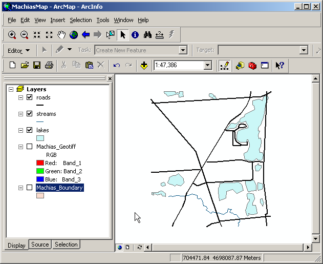
When you are done editing choose Stop Editing from the Editor menu. Hide the geotiff image and you should see that you have created a new vector map from the image!
Adjust the properties of the vectors to get the colors you want. You may use the standard symbology if you wish.
Here is what mine looked like:
Now create a final map in Layout view. As you have done this before with the HBEF geologic map, you should be able to do this without guidance.
When your map is finalized, publish it on your web page as before.