Exercise Data

The two DEMs that include the Mars Rover landing sites cover 0º to 44º South latitude and 90º to 180º and 270º to 360º East longitude. Smaller cropped versions (17 MB) of the DEM tiles were generated and included the class directory. Copy the tarballed lesson dataset from the directory MERData in the class data directory. Unzip it into your own class directory.

Adding and Displaying the DEMs

Because the landing sites are far apart relative to the extent of the DEM, you will create two dataframes, one for Spirt and the other for Opportunity. Start ArcMap. Name the available data frame Spirit. Remember that you can only work in one Data Frame at at time. To make a data frame active, right click on it and choose "Activate".

Make the Opportunity frame active and add the opportunity_mer_b_moladem.tif DEM. Zoom to layer to fill your screen with the DEM. Right-click on the image and choose Properties. Click the Symbology tab and select Histogram Equalize to set a good color stretch, and choose the color ramp that ranges from white through pink to dark orange or the white to dark red color ramp that also displays the DEMs nicely.

Go to the Tools main menu and Extensions. Click on the box to activate Spatial Analyst. Under View, turn on the Spatial Analyst toobar. In the Spatial Analyst drop-down menu choose Surface Analysis > Hillshade, and use the default hillshading settings. Drag the original DEMs above the hillshades in the Table of Contents and, in the Properties Display tab, set their transparency level to 50 percent. In the Proprites dialog under the Symbology tab, use a standard deviation stretch with a power of 2 on the hillshade to apply a contrast stretch on the image.

By "coloring" a hillshade like this you can create a 3-D effect while still communicating quantitative information. The data in the tif image correspond to elevation relative to the range of the etnire dataset. The minimum and maximum topography observations within the current data set are -8208. meters, the bottom of a crater in Hellas at 62.2E 32.9S, and 21300 meters at 226.6E 17.36N, the edge of a crater on the south rim of Olympus Mons.

Create another Data Frame called Opportunity and repeat the process above so that you have two DEMs.

Adding MOC and THEMIS Imagery

All sample data images have been geometrically projected into an equidistant cylindrical projection. Some images will cover Spirit's landing site, and the others will cover Opportunity's landing site.

1. Start building up the image layers by adding all the JPEG files from the themis_moc/directory.
2. In ArcMap, right-click on the name of each image, choose Properties, click on the Symbology tab, and check the box next to Display Background Value and make sure the value is 0. JPEG compression causes a slight black fringe on the sides of the images. A value of 0 for the background value will cause these black edges on the images to display as no color.
3. Arrange the images so the ones with the largest spatial extent are near the bottom Table of Contents.

The Spirit landing site contains three types of images—THEMIS daytime infrared images, THEMIS visible images, and MOC images mosaicked together. The largest image, I00881002RDR.jpg, is a THEMIS daytime infrared image. This image is in the 9th infrared radiation (IR) band at 12.57 microns, has a spatial resolution of 99 meters per pixel, and is actually a measurement of temperature. The sunlit slopes are warm and bright, and the shadowed slopes are cold and dark. V00881003RDR.jpg, the next image, is a THEMIS visible image at 0.65 microns and a resolution of 17.4 meters/pixel. Both THEMIS images were made available courtesy of NASA, the Jet Propulsion Lab (JPL), and ASU. Spirit's last image, r1303051_r1301467_50_rectify.jpg, is two MOC images mosaicked together at a resolution of 1 meter per pixel and provided courtesy of NASA/JPL/MSSS. To fit the basemap, it was slightly rectified.

For each of the images, provide a short description of the dataset in the General tab of the properties dialog. You may cut and past the text from above if you wish.

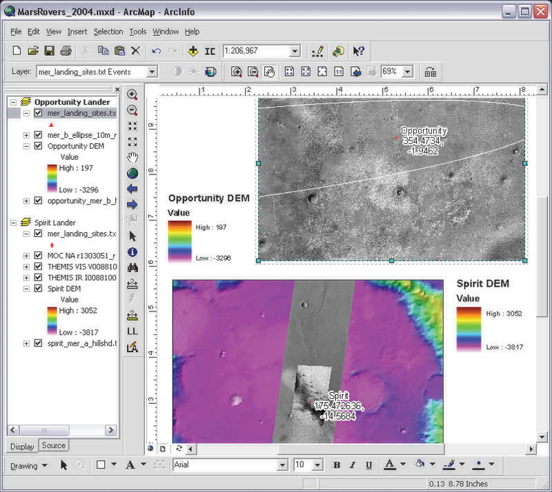
An ArcMap layout showing the MOLA and image layers with the landing sites plotted as points

The main image for the Opportunity site, mer_b_ellipse_10m_rectify.jpg, is a mosaic of THEMIS visible and MOC images and was resampled to a 10-meter/pixel resolution. The error ellipse plotted in the middle of the image defines the extent of that area where the lander could have come to rest. This image was created by MSSS and has been made available courtesy of NASA/JPL/MSSS/ASU. After plotting the landing site, you will see that the engineers did an excellent job of targeting the lander within the ellipse. To fit the basemap, this image was also slightly rectified but still contains some registration errors in the MOLA and MOC images.

Setting a Mars Projection

Before plotting the landing site locations, the data frame projection needs to be set. Although a Mars geographic definition is available in ArcGIS 9, for this exercise, a predefined Mars projection file called Mars_2000Sphere.prj was supplied in the sample dataset. Right-click on the data frame name and choose Properties. Click the Coordinate System tab and select New > Projected Coordinate System. Type in a meaningful name and set the values as shown below in Figure 1.

In the lower half of the dialog box, under Geographic Coordinate System, click the Select button and browse to the directory where you unzipped the sample dataset. Choose Mars_2000Sphere.prj and click Add, then click OK to set the projection for the data frame. To use this projection again, click the Add to Favorites button before clicking OK again to close the dialog box. Repeat this process for both data frames.

Plotting the Landing Site Coordinates

The rover locations were determined by the MER navigation and science teams by fitting direct-to-earth (DTE) two-way X-band Doppler and UHF two-way Doppler between the rovers and the Mars Odyssey satellite and matching features in satellite images to images returned from the rovers. With respect to surface features, the Spirit lander is located at 175.4729ºE, 14.5692ºS, and the Opportunity lander is located in a ~20-meter diameter crater at 354.4734ºE, 1.9462ºS. These locations are not exact, and as more information is returned, they could change. For this exercise, the Spirit values will be slightly shifted to 175.472636ºN, 14.5684ºS so they will better fit the images. For additional information on methods for locating the rovers, visit the MSSS site at www.msss.com/mer_mission/finding_mer.

1. To plot the landing locations, create a text file and name it mer_landing_sites.txt. Type the text in Figure 2 exactly. Save and close this file.

   Lander, Longitude, Latitude Spirit, 175.472636, -14.5684 Opportunity, 354.4734, -1.9462 Figure 2: Text for mer_landing_sites file

2. Using the Add Data button, add the file mer_landing_sites.txt to the Opportunity data frame.
3. Right-click on the file name and choose Display XY Data. In the Display XY Data dialog box, set the X Field as the Longitude and the Y Field as the Latitude. Click the Edit button. Before these points can be drawn correctly in an equidistant cylindrical projection, these points need to be defined on Mars.
4. In the Edit dialog box, click the Select button and browse to the directory where you unzipped the sample dataset. Choose the file Mars_2000Sphere.prj again and click OK twice to exit. Once the file is added, feel free to change the symbol and label options for the map.
5. Once the symbology is how you like it, copy the Landing Sites feature class to the Spirit dataframe so that it appears in both dataframes.

After the landing site points are plotted, zoom into the Spirit landing site on the MOC 1m resolution image. Notice the white area under the lander's location. Another white area is northwest of the Spirit lander. The white mark, near the middle of the image, is actually the lander. The northwest white area is the parachute and backshell that detached from Spirit during descent. Also notice the dark scar on the rim of the crater to the northeast. This is believed to have been caused by the impact of the detached heat shield, which was also released during descent.

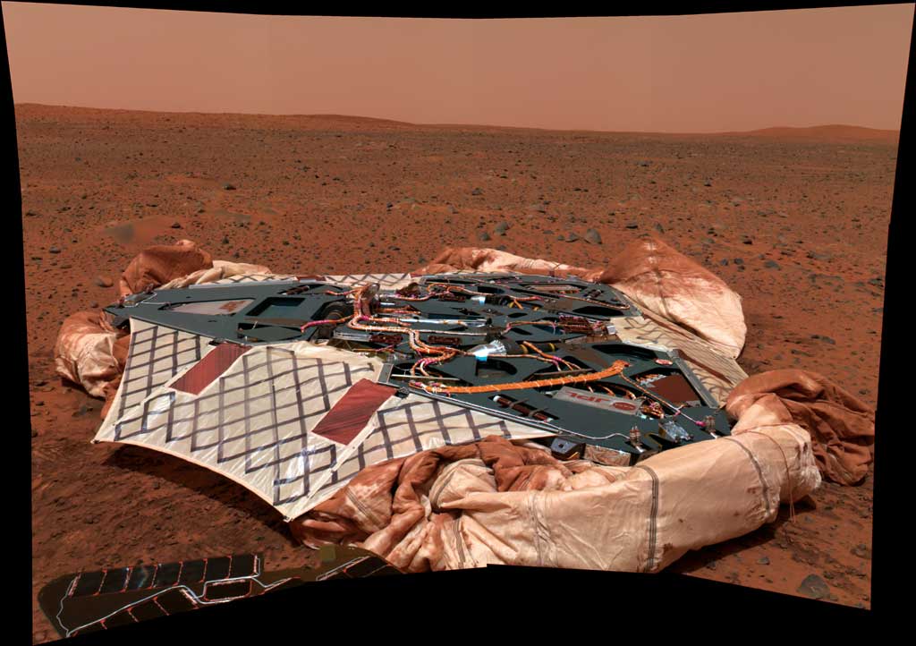This image mosaic taken by the panoramic camera onboard the Mars Exploration Rover Spirit shows the rover's landing site, the Columbia Memorial Station, at Gusev crater on Mars. This spectacular view may encapsulate Spirit's entire journey, from lander to its possible final destination toward the east hills. On its way, the rover will travel 250 meters (820 feet) northeast to a large crater approximately 200 meters (660 feet) across, the ridge of which can be seen to the left of this image. To the right are the east hills, about three kilometers (two miles) away from the lander. The picture was taken on the 16th martian day, or sol, of the mission (01/18/19, 2004). A portion of Spirit's solar panels appear in the foreground. Data from the panoramic camera's green, blue, and infrared filters was combined to create this approximate true color image.

The highest resolution image for the Opportunity lander site is called 01_overview_nolabled-B016R1.jpg. This MOC image has a resolution of 1 meter per pixel and contains the white pixel marks showing the lander (left of middle in the small crater) and the parachute and backshell near the western edge. The heat shield scar is in the southeast in the image and directly south of the large crater. This image is courtesy of NASA/JPL/MSSS.

You will be asked to propose a path for Spirit to visit the large crater that appears as a dark spot at 175º31'17"E 14º35 '41"S. Create a new line feature class with the correct projection and edit a proposed path for the Spirit to take to the site. Try to visit interesting features along the way based on the information you have.

To Turn In

You will need to turn in two maps.

The first shows the available data in a coherent manner. You can use the above image as a guide, but try to design your own layout to display the data according to your own interests.

The second map shows proposed path of the Spirit rover. Use the drawing features in Layout to label points of interest along the way and the cumulative distance along the path (e.g. potential outcrop, 137 m). Create a map with appropriate scale and annotation to display the path.

WHEN YOU ARE FINISHED, you can see that actual path that the rover took. No cheating!

Publish both maps on your web site for review.

Back to Page 1