Image inhancement describes the manipulation of images to improve intepretation. Image enhancement is distinguished from image processing, which better describes corrections to the image before they are intepreted (e.g. geometric or radiance corrections).
Before you start the lesson you need to complete ENVI 3.5 Tutorial #2. Note that you may have trouble with the last step, saving an image to GeoTiff format. If you get an error when you try to save, skip that step.
In this lesson you will perform image enhancements and filters to some example images. These tools allow features of interest in the image to be highlighted, and therefore better interpreted.
You will use an image of the Susquhanna River and another of the Jovian moon, Europa. Both are all located in the class directory:
/nsm/class/gly560/class/enhance
Contrast stretching is used to enhance different portions of the spectrum. Data are stored in 8 bit format, so that intensity is always displayed on a scale of 0 to 255 (256 levels of intensity). In your tutorial, you should have learned how to manipulate images with the ENVI Tools. We will apply these methods to help delineate a thermal plume in a River.
The image you will be using is an nighttime ASTER thermal image aquired on 2001-09-13, of the Susquehanna River, near the Pennsylvania/Maryland border. Band 10 has been extracted from the data set. The dataset is in ENVI format, so you can open it simply as a Data file.
A power plant near Coyne Locks discharges coolant water into the Susquehanna River, upstream of the Conowingo Dam. Use the contrast stretching techniques you learned in the tutorial to find the thermal plume from this power point. In thermal images, lighter colors represent warmer areas. Later in the class, we will learn how to extract temperature from these images, but for now, assume that temperature varies linearly with pixel intensity. Once you identify a thermal anomaly in the river, a good trick is to zoom in on the locale, and then contrast stretch using the zoom window as reference.
Use Density Slice to select data ranges and colors for highlighting areas in your grayscale image.
1. From the Display menu, select Tools > Color Mapping > Density Slice or Overlay > Density Slice.
The Density Slice Band Choice dialog appears. It lists all of the bands that have the same spatial size as the image in the display window.
2. Select the band to use for the density slice data ranges by clicking on the bandname.
3. Accept the default color table, and click OK.
Can you better identify the plume from this image?
Use the profile tool to create a profile of pixel intensity (temperature) along the river. You will need to define an arbitrary profile. From the Tools menu, select Profile -> Arbitrary Profile, and define a profile along the centerline of the river. Right click to finish the profile, and again to finish. A window should pop up with a transect of the pixel intensity along the profile you defined. Left click on the profile and drag the crosshairs along the profile. You should be able to locate the position of greatest temperature in the river using this tool.
You are finished with the Susquhanna River image at this point, so you can close all the active files.
Aside from considering the overall pixel distribution, we can consider the spatial distribution of pixel intensity in a remotely sensed image. Thus, we talk about the spatial frequency of an image, defined as the number of changes in brightness value per unit distance for any particular part of an image (Jensen, 1996). To enhance features within an image, we can perform spatial filtering, to remove or enhance particular spatial frequencies. We will consider two types of spatial filtering here, Convolution Filters, and Fast Fourier Transforms.
Convolution is a form of filtering that produces an output image in which the brightness value at a given pixel is a function of some weighted average of the brightness of the surrounding pixels. Convolution of a user-selected kernel with the image array returns a new, spatially filtered image. General requirements for configuring and using convolution filters and specifics for each filter type are described below.
|
Convolution filters produce output images in which the brightness value at a
given pixel is a function of some weighted average of the brightness of the
surrounding pixels. Convolution of a user-selected kernel with the image array
returns a new, spatially filtered image. You can select the kernel size and
values, producing different types of filters. Standard filters include high
pass, low pass, Laplacian, directional, Gaussian, median, Sobel, Roberts, and
user-defined. For descriptions of each filter type, see Convolution Filters.
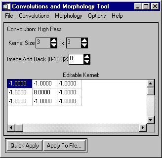
High Pass Filters
High pass filtering removes the low frequency components of an image while retaining the high frequency (local variations). It can be used to enhance edges between different regions as well as to "sharpen" an image. This is accomplished using a kernel with a high central value, typically surrounded by negative weights. ENVI's default high pass filter uses a 3 x 3 kernel with a value of "8" for the center pixel and values of "-1" for the exterior pixels. High pass filters can only have odd kernel dimensions.
Low Pass Filters
Low pass filtering preserves the low frequency components of an image, which smooths it. ENVI's default low pass filter contains the same weights in each kernel element, replacing the center pixel value with an average of the surrounding values. The default kernel size is 3 x 3.
Laplacian Filters
A Laplacian filter is a second derivative edge enhancement filter that operates without regard to edge direction. Laplacian filtering emphasizes maximum values within the image by using a kernel with a high central value typically surrounded by negative weights in the north-south and east-west directions and zero values at the kernel corners. ENVI's default Laplacian filter uses a 3 x 3 kernel with a value of "4" for the center pixel and values of "-1" for the north-south and east-west pixels. All Laplacian filters must have odd kernel sizes.
Directional Filters
A directional filter is a first derivative edge enhancement filter that selectively enhances image features having specific direction components (gradients). The sum of the directional filter kernel elements is zero. The result is that areas with uniform pixel values are zeroed in the output image, while those that are variable are presented as bright edges.
Gaussian Filters
A Gaussian filter passes a Gaussian convolution function of specified size over the image. The default is a 3 x 3 kernel and kernel dimensions must be odd.
Median Filters
Median filtering smooths an image, while preserving edges larger than the kernel dimensions (good for removing salt and pepper noise or speckle). ENVI's Median filter replaces each center pixel with the median value (not to be confused with the average) within the neighborhood specified by the filter size. The default is a 3 x 3 kernel.
Sobel Filters
The Sobel filter is a non-linear edge enhancement, special case filter that uses an approximation of the true Sobel function, and is a preset 3 x 3, non-linear edge enhancement operator. The size of the filter cannot be changed and no kernel editing is possible.
Roberts Filters
The Roberts filter is a non-linear edge detector filter similar to the Sobel. It is a special case filter that uses a preset 2 x 2 approximation of the true Roberts function, a simple, two dimensional differencing method for edge-sharpening and isolation. The size of the filter cannot be changed and no kernel editing is possible.
User-Defined Convolution Filters
You can define custom convolution kernels (including rectangular rather than square filters) by selecting and editing a user kernel.
Fourier analysis is a mathematical means of separating an image into its various spatial frequency components. In essence, it says that an image with a spatial distribution of pixels can be equivalently represented by the superposition of different spatial frequencies. When we make a forward Fourier Transform, we move from spatial coordiates in x and y, to frequency coordinates of magnitude and phase. All of the information of the original image is contained in Fourier space, and can be transfered back into the spatial domain using an inverse Fourier Transform. The numerical algorithm used for this transformation is called the Fast Fourier Transform of FFT.
In practice, a Fast Fourier Transform (FFT) is used to transform the data into a complex image that emphasizes the frequency distributions. FFT filtering in ENVI, selected from the Filters pulldown menu, consists of the forward FFT of an image, interactive building of frequency filters, application of the filter, and the inverse FFT transform to the original data space. Presently, FFT processing does not use the ENVI tiling procedures, so the size image that can be processed is limited by the available system memory. FFT images, which are "Complex" data type use eight times the memory of a byte image of similar size.
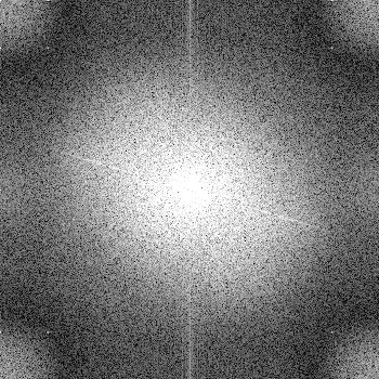
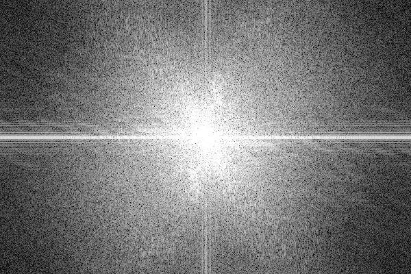
To perform a FFT filter, one masks out certain sections of the Fourier image and then inverts the image back to the spatial domain. The portion masked represents those spatial frequencies that one does not want to appear in the final image. This is used for filtering out banding and other signal noise, for example. In the image below, the Fourier represenation of single frequency noise signals at right, is shown at left. This image is the magnitude portion of the Fourier transformed image. The Fourier magnitude images are symmetric about their center, and u and v represent spatial frequency, where u is the horizontal axis and v the vertical axis. The image is by convention adjusted to bring the zero frequency to the center of the image, so that low frequency components are near the center of the image and high frequency components are near the edges. The Fourier images below consist only of points, because there is only one spatial frequency in the image.
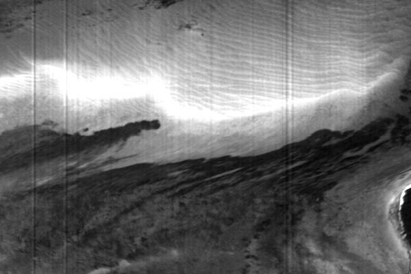
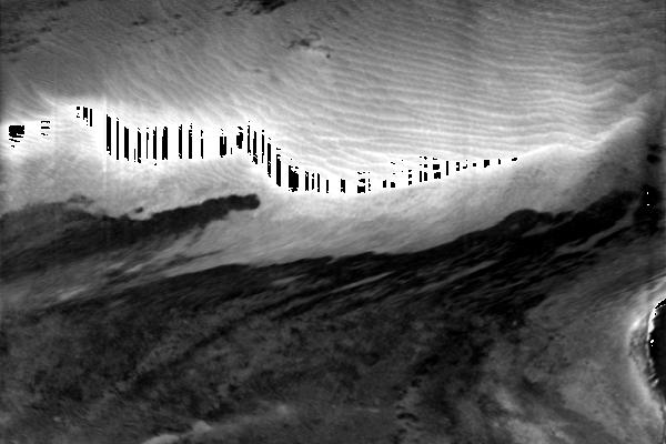
If these bands were superimposed on an image, they could be removed by removing the points from the Fourier image, and then inverting. For example, the image below of sands in the bahamas displays banding. The Fourier image is below. Notice the horizontal band that represents vertical banding in the image, over a range of frequencies. Banding can be removed by masking the this horizontal band and performing a Fourier inversion. The result is that the banding is removed form the image as shown in the bottom image. Unfortuntately, such filtering can also remove wanted frequencies that result in artifacts. This is also shown in the bottom image. The bahamas image is found in the class directory, if you want to play with it.
We will try filtering an image of the one of the Galilean Satellites, Europa. The surface of Europa is quite smooth with few markings (minimal craters) other than the pronounced sets of darker brown "fractures" that divide the crust into polygonal segments. These cracks are only slightly higher or lower (<300 m [984 ft]) than the main surface that appears to be water ice, which may top an ice-water slush or a pure water "ocean" at some depth before grading again into ice and then rocky material.
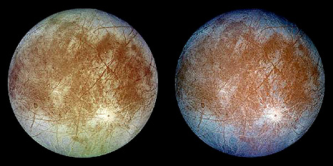
Open the ENVI image data file Europa for the following exercises. The data file can be found in the class directory.