Introduction to GIS Maps: ArcMap
In this exercise you will work with a Geology Map of the Hubbard Brook Experimental Forest, in the White Mountains of New Hampshire. The Hubbard Brook Experimental Forest (HBEF) is a 3,160 hectare reserve located in the White Mountain National Forest, near Woodstock, New Hampshire. The on-site research program is dedicated to the long-term study of forest and associated aquatic ecosystems. The HBEF was established by the USDA Forest Service, Northeastern Research Station in 1955 as a major center for hydrologic research in New England. These data were obtained from the HBEF data web site.
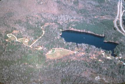
This coverage was obtained in digital form from Chris Barton of the USGS. Bedrock geology in the Hubbard Brook Valley was mapped by C.C. Barton, R.H. Comerlo, and S.W. Bailey, August 1994 to August 1995. The Map is entitled "BEDROCK GEOLOGIC MAP OF HUBBARD BROOK EXPERIMENTAL FOREST AND MAPS OF FRACTURES AND GEOLOGY IN ROADCUTS ALONG INTERSTATE 93, GRAFTON COUNTY, NEW HAMPSHIRE" and was approved for publication on August 28, 1995.
You can view a large (3MB) pdf version of this map.
First, create a folder in your class directory /nsm/class/geology/gly560/class/username entitled “IntroGIS”. Then go to the class directory, /nsm/class/geology/gly560/class and in the directory HBEF_Geology, find the tarball file hbef.tar.gz. Copy the tarball data file into your new directory. Extract the data into your folder. List the files that you just extracted. You should have files with root names of contx, faults, hydro, roads, strux. For each root name, there should be a .dbf, .shp, and .shx files. We will discuss what the files are at a later time.
Open ArcMap. Choose to
create “A New Empty Map” when asked. Add new data by pressing the ![]() button.
Navigate to your data file and add all the files that you see there (you can
select multiple files using the shift key). Choose “Add” and you should see
the files appear in the table of contents at the left of the screen. All of
the layers will come up as maps in the display window.
button.
Navigate to your data file and add all the files that you see there (you can
select multiple files using the shift key). Choose “Add” and you should see
the files appear in the table of contents at the left of the screen. All of
the layers will come up as maps in the display window.
Before you go any farther, save the project in your class IntroGIS folder. Under the file menu choose “Save As.. “ and save the project file as HBEF_Geology.
Notice as you move your point around the map, the coordinates are listed at the bottom. This map is designed to have coordinates in degrees (geographic coordinates). Other maps may be projected into another coordinate system such as Universal Transverse Mercator (UTM).
Select and unselect the map layers so you can differentiate the layers. You will notice point, line, and polygon shapes. Strux shows outcrops where structural observations have been made, faults are fault locations (only one shown), roads are the major roads at the site, hydro is hydrology (only Mirror Lake is displayed), and contx are the geologic contacts.
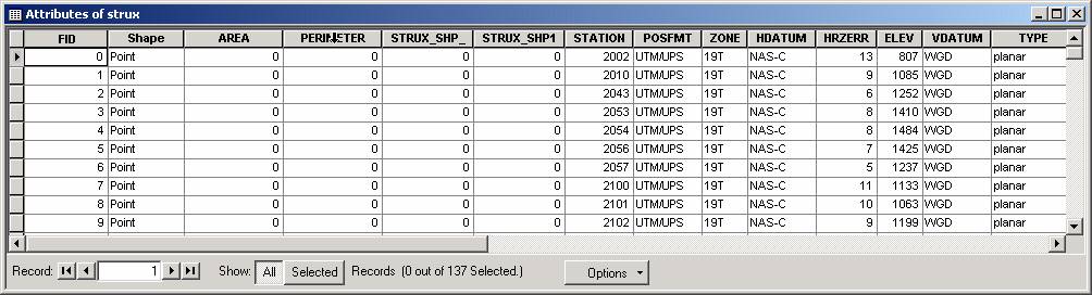
Right click the contx layer and open the attribute file. The attribute file contains all the information associated with these points on the map. The first column is a unique id for each feature (FID), the second the type of shape, then some geometry attributes which aren’t used because these are points, and then the geologic data. Scroll right and you will see various information that geologist thought important including their own station identifier, elevation, the type of feature (planar, linear), strike, dip. There is also information about symbology which we will not address in this exercise.
Open the attribute files of the other layers to see what data are associated with the map layers.
In this form, the map doesn’t look much like a geologic map. We need to make some edits to the display of these features to make it more meaningful. First, rearrange the layers so that the polygons are below the point and line shapes, so they don’t cover them up. Drag the contx layer below the others in the table of contents.
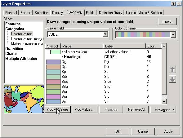
Right click on the contx file and choose Properties… Then chose the symbology tab. Right now, all the polygons are depicted identically. We want each formation type to appear with a different color. Chose “Categories” and “Unique Values”. Under Value Field choose Code, which is the code for the formation names in the map. Under color scheme, choose a relatively neutral color so it doesn’t overwhelm the point and line features. Descriptions are not available in this file, so we will treat these generically for the moment. See the hard copy map on display for more info.
Notice that the lake is covering some the geology contacts. Right click on the hydro layer and change the symbol to “Hollow” choose appropriate line thickness and color so that the lake is still visible but it no long obscures geology.
The names on each of the layers are abbreviated because they have been taken from the file names. We would like to have something more descriptive. Right click to edit Properties again, and choose the General tab. Notice you can change the layer names. Change the names to Geologic Formations, Hydrography, Roads, Outcrops, and Faults.
In this “Data” view, you can work display data in different manners, make queries, and manipulate attribute data. It is not designed to make hardcopy final maps, however. For this, we want to switch to “Layout” view. From the main menu, under View, select the Layout View. Notice how you now see a “print format” view. A blank page is automatically shown with the map that you are creating on the Data view. We will annotate this map to create a final version of the geologic map.
Click on the “Insert” menu item at the top of the page. You will see a variety
of annotations that can be added to the map. As you know, a map is meaningless
without basic reference information like a title, legend, scale bar, north
arrow. You will add these features to your map now.
First, add the north arrow. Choose north arrow and you will see a menu selection of north arrows. Chose the one that suits your fancy and click OK. It should appear on your map. You can drag and place it where you wish. You can also drag the corner of the arrow box to resize.
Now add a scale bar to the map. Drag it to where you would like on your map. Note that the scale bar comes across in Degrees, which isn’t terribly helpful. We will see how to change this when we work with coordinate systems later on. For now, make the scale bar a comfortable size by dragging the corner. Notice that the object is not merely resized, but actually maintains the correct scale.
Next add a legend to the map. ArcMap will take you through a wizard to help you customize the legend to your liking. It allows you to choose which layers you want to include in your legend, and the order in which they are presented. Choose the default values throughout the wizard. It will place the legend on your map, but you will need to shrink the map itself to find space for it, probably at the right of the map.
Finally, add a title to your map in the same manner as the other attributes. The title should reflect the name of the data (e.g. Geology Map of the Hubbard Brook Experimental Forest) not the exercise.
Insert some small text at the bottom of the map that indicates the date the map was created and the author (your name).
Save your project file.
Finally, we want to export the map so that you can turn it in. Under the main menu go to File… Export Map. Under Type, you will see that you can choose from a large number of graphics files. For maps that contain sharp lines (vector data) the compressed image formations like jpeg and gif do not work well. You can save as a Encapsulated Meta File (EMF) and put it in a Word document, or export to Adobe Illustrator and usually get good results. Since we want to publish this project on the web, we had better use a more general format like Tiff (.tif). Save your map as a .tif file.
Copy the map to your public_html folder on your home directory. To turn the map in, create an html document in your public_html folder entitled gly560_assignments.html. Create a link in this page called “HBEF Geology Exercise” that links directly to the digital version of your map. When you click on the link, the map should be displayed.
You’re Done!