You will import two geologic maps of western New York, available at the State Museum of New York GIS Dataset Site. You will work with these maps to get them into a summary form, and make a few calculations based on the final maps.
The most common way to distribute ESRI-based GIS data is through the Arc/Info Interchange File format. These files are easily recognized by their suffix, enn (or Enn) where nn is a number from 00-99. If only one coverage was exported from ArcInfo, then the suffix will simply be .e00 or .E00. Although interchange files were created with ArcInfo 7.x, they can be imported into ArcView using an import utility. On an NT-based ArcView 3.x program, you can use the IMPORT71 utility that is found in the same folder as the ArcView program, and is usually installed in the same menu as ArcView. This program will efficiently import interchange files into a data source in a format that can be added to a project or view in ArcView. For Unix based systems, you can use the IMPORT utility to import interchange files.
Prepare a directory in your class directory, called niagara_geol. Create subdirectories called "data" and "shapefiles".
Go to the New York State Museum web site GIS data page. Page down until you find the Surface Geology Niagara Sheet data, and download the .e00 version of the map (niag_s.zip.e00) into your data directory. Also download the metadata file, and at the top of the table, the "Surficial Geology Legend: Explanation of surficial materials" grouped by depositional environment, in HTML format.
Scroll down to the Bedrock Geology maps. Into your data directory, download the Niagara sheet data (niag_bedr1a.zip) and from the top of the table the "Explanation of Bedrock Materials" text file.
In case the New York State Museum web site GIS data page is down, you can obtain these files from the class directory under the directory niagara_geol.
Both of the interchange files you downloaded were compressed using a DOS program called PKZIP. To unzip on a UNIX machine, you need to use gunzip. To use gunzip, you will need to rename the files from *.zip to *.e00.gz. Then you can use the gunzip command to uncompress the files.
Uncompress both files using gunzip into your data directory.
You will need to extract the data (import to ArcView) from the interchange format, before it can be added to your ArcView project. This is done on UNIX using the IMPORT command. This utility is located in the same /bin directory as ArcView, but should be available.
Before we can use IMPORT, however, we need to set the environment variables. The easiest way to do this is to run ArcInfo, even though we won't actually be using the program.
Now we can use the import command. While still in your data directory, open a console window and type:
import [interchange_file] [output]
where
[interchange_file] is the name of the interchange fileFor example, to import niag_s.e00, you would type:
/eng/tools/esri/arcview3/bin/import niag_s.e00 niagsurf
This will create two directories in username:
/nsm/class/gly560/username/niagara_geol/data/niagsurfArcInfo coverages always contain an "info" folder in addition to the files in the coverage folder. When you import the bedrock interchange folder, it will add additional files to the info folder, but that's OK.
Import the other interchange file following the steps above.
You should now have three folders: one for the bedrock geology, one for the surface geology, and an info file. Your data are now imported and we are ready to start the ArcView project.
Begin a new ArcView project, name it niag_geology, and save it in your niag_geology directory. Set the working directory to your shapefiles directory. To a new view, add the bedrock coverage that you created in the data directory. Name the view Bedrock Geology.
At this point, you will want to save the bedrock coverage as a shapefile. Convert the theme to a shapefile in your shapefile directory under the name "niagbed". Rename the theme Bedrock by Formation. Save the project.
Open the attribute table for the bedrock coverage and you will see that along with polygon information (area, perimeter) there is a Material field. Open the text file that you downloaded "bedrock.txt" and you will see that the material designations correspond primarily to Formation names, but also some more general geologic descriptions.
If you activate the bedrock theme you will notice it is all one color. Open the legend and change the Legend Type from Single Symbol to Unique Value, and choose Material for the values field. Use "Minerals" for the color scheme.
Save the project.
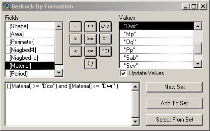
We want to classify this map in terms of Geologic Periods. By now, you should know how to use the query builder to create new themes. To classify this map in by periods, we could query the formation names by period (see below) and then build new sets, then themes, for each period.
However, we will try a different way to classify by periods. We will use the Field Calculator to create a new classification field called "period" and create a new map based upon that classification.
Open up the table for Bedrock by Formation, and begin and edit session. Create a new field string called "Period", and allow it to be 16 characters long. Using the field calculator, we will extract the first letter of the formation name to determine the period. Activate the Period column and start the Field Calculator. Find the string expression "Left". The expression operates as follows:
LeftMake sure that none of the records (or all) are selected using the ![]() button, and use this expression to place the first character of each entry in
Material in the field Period, followed by the "_" character. The field
calculator expression should look like this:
button, and use this expression to place the first character of each entry in
Material in the field Period, followed by the "_" character. The field
calculator expression should look like this:
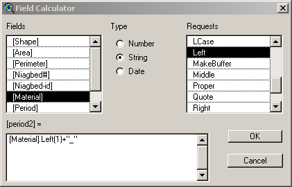
This command should populate every entry in the field with the first letter from the Material column followed by "_", e.g. "D_" for Devonian. Now we want to convert these letter designations to actual Period names. To do this, we can use another field calculator command "substitute". The usage of substitute is as follows:
Substitute
Substitutes each occurrence of matchStr in aString with replaceStr and returns
the new string.
Usage: aString.Substitute (matchStr, replaceStr)
This time, however, we want to perform the string operation in place. If we created another column and tried to perform multiple substitutions, subsequent substitutions would overwrite previous substituions. Before we do this, save your edits to the table thus far.
Select the Period column and activate the field calculator. Use the substitute expression to substitute "Silurian" for "S_":

This operation should replace all "S" values with "Silurian". Repeat this process for all other periods and substitute "Water" for h2o. The reason we used the "_" after the letters, was to avoid replacing text already in a period name with another period (e.g. you might end up with "MississiPennsylv"). Save your edits, stop editing and close the table. Save your project.
Make sure to unselect all records in the attribute table (use the ![]() button)
and convert the theme to another shapefile called "niagperiodform".
Add the new theme to the view and rename it "Bedrock Geology by Period
and Formation". Use the legend editor to classify the Period names and
use Fruits and Vegetables as the color scheme. Notice that the order of the
Periods in the legend is not top-down, youngest to oldest, as it should be.
Rearrange the periods from top-down, youngest to oldest. Do not even think about
asking the instructors in what that order they should be. Put water at the bottom
and change it's legend color to light blue. Save the project.
button)
and convert the theme to another shapefile called "niagperiodform".
Add the new theme to the view and rename it "Bedrock Geology by Period
and Formation". Use the legend editor to classify the Period names and
use Fruits and Vegetables as the color scheme. Notice that the order of the
Periods in the legend is not top-down, youngest to oldest, as it should be.
Rearrange the periods from top-down, youngest to oldest. Do not even think about
asking the instructors in what that order they should be. Put water at the bottom
and change it's legend color to light blue. Save the project.
Notice that your map still shows lines that separate all of the formation names. As we are only interested in the Periods, we will "dissolve" the boundaries among the the formations using the Geoprocessing Wizard.
Go to File...Extensions.. and check the Geoprocessing Wizard. Under view, start the Geoprocessing Wizard. Select "Dissolve features...", choose "Bedrock Geology by Period and Formation" as the theme, and Period as the attribute to dissolve, and select the output file as "niagperiod". The next window allows you to choose a fields that you may wish the Geoprocessing Wizard to calculate. Choose Area by Sum and any other calculations you think might be interesting and click Finish. Add the new theme to the view and rename it "Bedrock Geology by Period". Rearrange the legend again in the proper top-down order, and change the color scheme to something appropriate.
When you activate the theme you will notice that the formation lines are no longer shown. These have been "dissolved" by the Geoprocessing wizard. Open the attribute table and you will notice that the table also contains only period data.
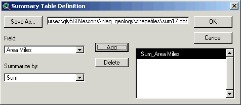
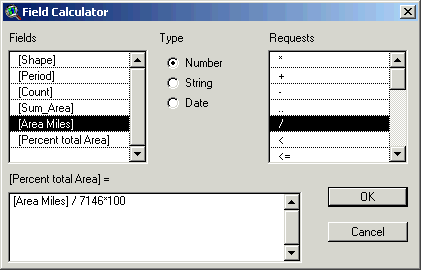
We will calculate the percent of the total area is represented by subcrop of each period. Open the attribute table for Bedrock Geology by Period for editing. Add a new field called Area Miles, 6 characters wide, with no decimal places. Populate the field with area in miles, by using the field calculator to convert the Sum_Area to in meters to area in miles (1 square mile = 2,590,000 square meters).
Now add a new number field called "Percent Total Area", six characters wide with 2 decimal places (the name will be truncated but that is OK). We want first to summarize the total area of the entire project. Unfortunately, the summarize function must group by a field. We will create a temporary field to calcuate a total area. Use the field calculator to populate the entire Percent Total Area field with the number "1". Then highlight the field, and click on the summarize button. Choose Area Miles as the field and summarize by Sum. Add this choice to the results window.
This action will summarize the values in the field Area Miles according to categories listed in Percent Total Area. Because there is only one category in percent total area, there is only one result, the total area of the region:
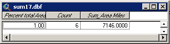
Now use this value of total area, 7146 miles, to calculate the percent area of all of the Periods and Water features. Use the field calculator to repopulate Percent Total Area.
Save your edits, stop editing the table and close the table. Save the project.
Finally, create a bar chart showing the distribution of all of the periods and water bodies as a fraction of the total area in the study region (for some reason pie charts do not work on the unix version of arcview). Show the map of the subcrops according to each period, with the chart. Title the final layout "Niagara Regions by Geologic Period. Title the chart "Per Area Distribution of Subcrop".
Save your project and layout. Turn in the final map for grading. You will be graded both on correct completion of the tasks above and map presentation (make it pretty and include all the essential elements of a geologic map).
In the previous example you classified a bedrock geology map according to geologic period. In the challenge, you will create a map of surface geology according to depositional environment. Material properties in the surface geology map are given in the "surface_type.html" file that you downloaded.
This time you will not be able to use the "substitute" command in the field calculator because the material indicators are not easily keyed to depositional type. You will need to create a second classification table by which the materials can be classified.
The easiest way to create the classification table, is to summarize the surface geology attribute table by "Material" and then open the resulting summarize table in Excel. In this way, you will start with a list of all material types. Given this list, create two more columns: "Deposit" that holds the name of the material type (e.g Colluvial Diamicton) and "Depositional Environment" that indicates the depositional environment (e.g. Till or Glaciocustrine). Type in the values for all of the material types, save the file in dbf form.
By joining the classification table to the surface geology table you will create a theme of depositional environment, and another theme that holds ONLY the depositional environment. To do this, use the dissolve feature as you did before.
Create a final map and layout similar to that you created for the bedrock map, showing the area distribution of the depositional environment in the project area.
As this is a "challenge" you will not be walked through this exercise but will need to figure out on your own, and with others in the class how to create this map and layout. Turn in the final map for grading. You will be graded both on correct completion of the tasks above and map presentation (make it pretty).