In this lesson you will begin to work with interpolation of data in ArcGIS. Later, we will examine how to interpolate data based upon a statistical analysis of data relationships in space (geostatistics). In this exercise, we will focus on some simple tools and get some practice with contouring.
You will correct, contour, and interpret gravity data. These data were collected by Mark Saunders, for his UB thesis in Geophysics. The study area is, of course, the Ischua Creek watershed which includes the town of Machias. In this lesson you will correct raw gravity data to identify gravity anomalies due to the variation in thickness of glacial valley-fill sediments. You will need to understand a bit about gravity surveys for this lesson and think about your data analysis. If you are not familiar with the processing of gravity data, you will need to read the provided excerpt from "Whole Earth Geophysics" by Robert Lillie.
You will need to create a "MachiasGravity" directory in your user directory. Within that directory, create two subdirectories: "data" in which you will store provided data for the exercise and "work" in which you will store the data that you create and manipulate. Copy the file MachGravData.tar.gz from the /nsm/class/gly560/class/MachiasGravity/ directory into the MachiasGravity/data directory. When you extract the files (using the gunzip and tar commands), it will create directories with the following files:
Create a new ArcMap project in your "work" directory called GravitySurvey. Add all the shapefiles in your Data directory. Check to make sure that the layer now has the coordinate system UTM 17N NAD27. This is the projection that we will use for this exercise.
The surficial geology map (surfgeo.shp) was digitized from a map by Frimpter (1974). The attribute table contains classifications of sediment types as described in the DESCRIPTION field. Classify the surficial geology by unique value using the DESCRIPTION field. Name the layer Surficial Geology.
Symbolize the subwatershed layer (subwshed.shp) as a hollow outline. Display the layer in the legend as "Ischua Creek Watershed Boundary".
Properly name and symbolize the roads and streams layers.
Add the 30m_DEM raster data to the map. As the name suggest this is a 30 m resolution digital elevation model for the watershed. It has been clipped to correspond with the Ischua watershed boundary. Give it a descriptive name in your map.
The raw gravity data are available in the Survey folder. It is provided as a dbase4 file (Gravity_Data.dbf). Add this table to your map. If you open the table you will see the coordinate locations for the data point, and the gravity measurement in mgal. The coordinate locations were determined from hand held GPS and are in WGS84 UTM 17N coordinates. You need to tell Arc that the XY data are in this projection.
Right click on the table and choose to Display XY values, choosing WGS84 UTM 17N as the coordinate system. You should notice that the "event" data points often align with roads along the sides of the valley, as the survey was taken at roadside locations. You will also notice that many of the gravity points are outside your watershed. We want to get rid of these. Use the Selection tool to select all points that are completely within the watershed boundary. Then right click the layer, choose Selection. Create Layer from Selected Features. This will add another layer to the feature class that contains only the points within the watershed.
Now we want to save these clipped data as a shapefile. Use the Export Data command to create a new shapefile for the gravity data. Name this new feature class "Gravity_Survey" and choose the same coordinate system as the dataframe, which should be NAD27. Save the file to your "work" directory. Check its properties to make sure that it has NAD27 projection.
If everything looks OK, you can delete (remove) all the XY layers and tables you used to create your Gravity_Survey shapefile.
As you will see in the following sections, we will need the elevation of the gravity points in order to calculate gravity anomalies. We will extract these elevations from the the DEM. This will be done using a process called Zone Statistics. The Zone Statistics Tool calculates the statistics of raster cells that fall within defined zones, dictated by another "zone" raster. Zones are defined as a group of cells that have identical values.
We want to use this tools to extract elevations from the DEM raster and append it to the attribute table of the gravity data. To do this, we first have to convert the vector gravity points to raster, and then extract the DEM elevations for each gravity "zone". ArcTools actually does this all in one step, but you need to be aware of what is happing to get the result you want.
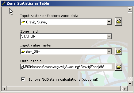
In ArcTools, open the Spatial Analyst... Zonal...Zonal Statistics as Table tool. This zonal tool is the choice when you want to create a table of zonal statistics. We will create the table then append it to our gravity survey attribute table. Open the tool. For the input feature use the Gravity_Survey shapefile. Choose the unique STATION as the zone field to create a new zone for every station number. The value raster is the DEM. Choose to output the table to your working directory (view window result). DO NOT START THE TOOL YET.
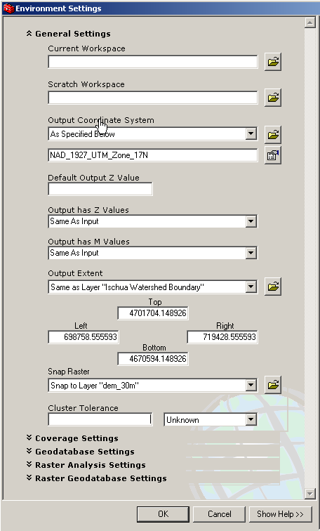
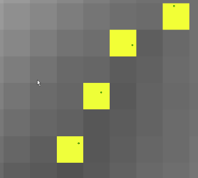
Before you run the tool, we will need to set the proper environments to make sure the zone raster and the value raster line up. Remember, Arc will create a raster from the vector data, and then use that to establish the zonal statisitcs of the DEM. If the two raster's don't mesh, the statistics appended to the Gravity Survey attribute table may be an average of mulitple DEM cells. This will result in incorrect elevation data. Open the Environments.. tab and expand the General Settings. Specify the output coordinate system to NAD27. Specify the extent as Same as Layer "Ischua Watershed Boundary" to make sure that the calculations cover our area of interest. Choose to Snap Raster to "dem_30m". This will force the rasterized Gravity Survey to coincide with the DEM. In the figure below, for example, the green cells are the rasterized gravity survey points, the points the gravity survey points, and the grayscale the DEM. This figure comes from creating the Gravity Survey raster manually. Check your environment settings against this example then close the environment dialog and run the tool..
You may need to add the created table to your project. Once you do so, you should be able to join the table to your gravity survey attribute table, using the station number (STATION) as your unique identifier. Right click on the Gravity Survey layer and choose Joins and Relates... Join... Join attributes from a table. Join your zonal table to the attribute table using STATION as the common attribute. When you open the attribute table you should see that statistics as additional fields. You will notice that the range is zero and the count is one because we average only one value by snapping the rasters together. The mean, then is the elevation data point.
Table joins are temporary, they are not saved when you exit Arc. Consequently, we want to permanently append the elevation data to the gravity survey table. To do this, we will create a field in the Gravity _Survey table, populate with the elevation data, and then remove the join. Under Options, choose to Add Field, name it Elev_m, and choose an Interger with precision 0. Acknowledge that you want to do this outside an editing session. Right click on the column heading and choose to calculate values. Input the values from the GravitySurvey.mean column. The column should now be populated with all the elevation data. Close the table and remove the join. When you open the attribute table again, the elevation data should still be there.
Zoom tightly in on one of the survey points in the uplands. Use the information tool to confirm that the survey point has extracted the correct elevation from the DEM.
<< Next >>