This web page was adapted from Spatial Hydrology Using ArcView 3.x, by David Maidment, Ph.D.
Geographic Information Data
A GIS presents spatial
information in themes. Each theme represents a data set for a defined
area. The geographic features are represented as points, lines, and polygons in
the two fundamental GIS data models, vector and raster.
The attribute information
for themes is stored in a spatial database. A GIS integrates common database
operations such as query and statistical analysis with the unique visualization
and geographic analysis benefits offered by maps and spatial databases.
Because the earth is curved
and maps are flat, a projection system needs to be used to transform the curved
earth into a flat map. People have always created maps of their world. Even the
most ancient map shows rivers and coastlines because water has always been the
most important natural resource. Modern
topographic maps include even more detail, such as roads, cities, and land
surface elevation using contour lines. Specialized maps are also constructed of
soils, land use and land cover, and other quantities. All map production makes
use of the idea of themes, or map layers. In GIS, the idea of themes as map layers is
transformed into themes as data layers. Each theme is a collection of similar
objects, such as individual road or stream segments, which are referred to
individually as geographic features.
Points, lines, and polygons,
In a data layer, the map
coordinates describing each geographic feature are stored. An individual point
is stored simply as a single pair of coordinates (x,y). A line is stored as an open sequence of points,
or vertices. By listing the vertices in order from one node to another, the
line possesses direction, so it is a directed line. The boundary of an area or
polygon is stored as a closed sequence of directed lines or as a closed
sequence of the vertices making up the boundary. The polygon boundary is closed
because the last vertex point is at the same location as the first one in the
sequence.
|
|
|
Illustration showing
point, line, and polygon vector data. [Click to
enlarge] |
Geographic features
represented as points, lines, or polygons are collectively referred to as
vector data objects.
A vector is a straight line
that has both a length and a direction. From a point of origin (0,0) in a coordinate system, a vector can be drawn to any
point (x,y). A vector, or line segment, can be drawn
between two points (x1,y1) and
(x2,y2). Similarly, for any number of points in a
sequence, a succession of vectors can be drawn between adjacent pairs of points
and thus collectively define a line of any appearance.
There is no such object in
GIS as a curved line such as is used in computer aided drawing systems (CAD) to
show a smooth curve around a road curbing. In GIS, curves are actually
represented as closely spaced sequences of line segments.
In addition to representing
geographic features using shapes, a GIS also uses symbols to provide more
information about the features. Point symbols often look like the features they
represent. Line symbols include thick or thin lines, solid or broken lines, and
may come in colors. Polygon symbols include the colors and patterns used to
fill in areas.
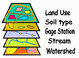
A spatial database is made
up of a collection of point, line, and polygon themes. Because this data
represents information about the earth, it is called geospatial data. The
graphic below shows some examples of geospatial data.
|
|
|
Themes, including vector
data descriptions, you might see in a map for hydrological analysis. |
Descriptive Attributes
When looking at a map, it is
helpful to know more about the features represented in it than simply where
they are. For example, when looking at a map of rivers and streams, it is
helpful to know their names. A hydrologist may want to know even more, such as
the slope of the river, the roughness of its bed and banks, and the shape of
its cross-section, because these qualities are important in being able to
define the velocity of water flow in the river.
This type of descriptive
information about a geographic feature is called its attribute data. Attributes
can be stored as numbers or character strings in a data record. A collection of
data records makes up a data table.
There are two descriptions
available for each geographic feature: its spatial location and its descriptive
attributes. It is essential for a GIS that these two descriptions be connected.
To do this, a unique identifying number must be associated with each geographic
feature. That number is then stored both with the spatial description and with
the attribute description.
For example, in the graphic
below, each of the water right locations on the map has its own unique
identifying number, so that the location of the water right on the map is
connected to the corresponding row in the attribute data table. This is called
a one-to-one
relationship.
|
|
|
Integration of spatial and
attribute information. |

A water right is a legal
permit for withdrawing water from a river or reservoir. Sometimes water rights
are progressively established, creating several water rights at the same
location. These individual water rights may be stored in a separate table and
connected through their location identifier, as shown in the above table. This
is an example of a one-to-many
relationship between one location and many objects associated with that
location. The attribute information may include the description of the water
right location, the owner of the water right, the stream on which the right is
located, and the rate of water withdrawal.
The spatial and attribute
information are linked, so you can get the attribute information by simply
clicking on the location on the map, or you can click on a water right in the
table and see where it is located on the map. The linkage of digital maps with
data tables distinguishes GIS from CAD and from relational databases such as
Oracle or Microsoft Access. A CAD system can produce the map; a relational
database can produce the data table; but only in a GIS is the one-to-one
linkage between the each map feature and the corresponding data record
achieved.
Vector and Raster Data
The discussion so far has
focused on geographic features in discrete space, where the objects are
spatially distinct from one another. An alternative view is continuous space
where a variable such as land surface elevation or precipitation is defined
everywhere throughout the study area. Continuous surfaces can be represented
using the grid or raster data model in which a mesh of square cells is laid
over the landscape and the value of the variable is defined for each cell.
As shown in the graphic
below, a point in a vector representation can be approximately transformed to a
single cell in a raster representation. Likewise, a vector line can be
approximately transformed to a sequence of raster cells lying along that line,
and a vector polygon can be approximately transformed to a zone of raster cells
overlaying the polygon area.
|
|
|
Comparing raster and
vector data. [Click to enlarge] |
Spatial hydrology involves
both spatial data development and hydrologic modeling. Each of these requires
intensive computational functions, which are usually offered by raster data
models. However, most spatial data sources are in vector data format, which
provides unique visualization and geographic analysis benefits. Therefore, the
coordination and connection between raster and vector data is critical in
spatial hydrology, perhaps more so than in other GIS applications.
Rivers are best represented
as lines, and gaging stations and other control
points on rivers, like water right locations, are best represented as points.
However, the watershed areas draining to those points are best derived from
Digital Elevation Models (DEM), which are raster representations of land
surface terrain elevation, a continuous surface.
Moreover, precipitation,
evaporation, and other climatic variables are defined continuously through
space and measured at particular points (e.g., climate stations).
Being able to move back and
forth smoothly between raster and vector representations of data is important
to spatial hydrology.
A well-constructed
geospatial database for hydrology incorporates both vector and raster data in a
tightly connected raster-vector data model, as illustrated in the graphic
below. The features of the real world are depicted in vector data layers as
points, lines, and polygons, and in the raster database as cells or zones of
cells.
|
|
|
Tightly-connected
raster-vector data model. |
While more spatially
approximated than the vector database, raster representation has one great
advantage. Unlike vector representations, which require different types of data
to be separated into different data layers, raster representation allows
various kinds of hydrologic features to be represented in a single grid.
Flat Map, Curved Earth
The earth appears to be a
sphere, but it is actually slightly flattened at the poles compared to the
equator, making it more of a spheroid, or ellipsoid.
Although the earth is a
curved surface, it must be depicted as flat to be presented on a map. The
process of transforming locations on the curved earth to corresponding
locations on a flat map is called map projection.
|
|
|
Map projections transform
locations on the curved earth from geographic coordinates into Cartesian
coordinates on a flat map. |
Locations on the earth's
surface are specified in geographic coordinates of latitude and longitude,
which are usually assigned the mathematical symbols Φ for latitude and
λ for longitude. Lines of latitude,
called parallels, encircle the globe with parallel rings, beginning with Φ
= 0° at the equator and increasing to Φ = 90° N at the North Pole and
Φ = 90° S at the South Pole. Lines
of longitude, also called meridians, stretch between the North and South poles,
beginning with λ = 0° on the prime meridian through
All locations on earth have
a latitude and longitude. For example, the location of
Flat maps in a GIS use
projected coordinates to map the earth's surface. Projected coordinates, also
called Cartesian or planar coordinates, are represented by the symbols (x,y), or easting and northing, in which x measures distance
to the East and y measures distance to the North, relative to the location of
the origin of the coordinate system.
Projected coordinates are
expressed in units of length, usually feet or meters, so distance and area can
be defined consistently throughout the domain.
Map projection is a
mathematical process in which, for all the coordinate points of each geographic
feature, the (, ) location on the earth's surface is
transformed to an (x,y) location on a map.
Some distortion of the
relative location of the points always occurs because a curved surface cannot
be exactly compressed onto a flat one. Some map projections preserve shape;
others preserve area, distance, or direction. No projection preserves all
properties. The following graphic indicates that the area has been distorted: