Back to Page 1
(note recent edits are shown in red)
Converting Data
For these data to be read by ArcMap, they will need to be
converted. This conversion will be accomplished by using various
scripts available in the ArcTools program. Our first goal is to
transform all data into shapefiles or raster datasets.
Import Hydrography Data
The hydrography data must be converted from ArcExport form.
ArcExport format was designed for older ArcInfo versions of the ESRI
software so it archives data in "coverage" form. The
process will be to convert ArcExport data to coverages, and then
coverages to shapefiles.
First, unzip the data into your HYD folder. You should be able to
do this without guidance by now.
Open up ArcTools from the ArcCatalog menu. So where is the tool to
import Arc Interchange files? This is a common problem with ArcTools,
just locating the right tool can be difficult. At the bottom of the
Arctool file tree window you should see tabs for Index and Search.
Try searching for e00, the suffix for the file. You should find that
the tool is located under the "coverage tools" category.
Start the tool for to "Import from Interchange File". Give
the tool the name of your downloaded *.e00 file from the CUGIR site
for the Delevan quad. Let the tool choose the other options and start
it. When it is finished, you should see a coverage in your
Delevan/HYD directory. This coverage has data called arc, node,
point, and tic. Previewing the data will tell you that it is the
"arc" that resembles the shapefile and is what we are
really after.
Covert the arc data to a shapefile by right clicking on the "arc"
data, choosing Export... and then to shapefile (single). Choose the
HYD folder for output and name the file delevanhydshp. Start the tool
and it should create the shapefile. Look at the
properties for this shapefile. Notice that the spatial reference
(under the Geometry Entry, remember) is UTM NAD27 18N. The spatial
reference has been retained with the conversion of the shapefile.
Change this projection to NAD27 17N to match the projection from your
previous Machias Map project. As you may recall, you can do this by
right clicking on the dataset, going tp properties, Field Tab, and
clicking on the Geometry properties under Shape. Click on the
elipses ... to select the new projection.
Now we want to import the metadata that you
downloaded from the site. Click on the shapefile in ArcCatalog and
choose the metadata tab. The metadata may have been imported when you
converted the coverage to the shapefile, but you will want to make
sure you have the correct metadata. Import the metadata from the XML
metadata file that you downloaded.
To import the metadata:
In the Catalog tree, click the
item for which you want to import metadata.
Click the Metadata tab.
Click the Import Metadata button
 on the Metadata toolbar.
Click the Format dropdown arrow
and click the format of the metadata that you will be importing. In
your case, you chose to use XML data..
Click the Browse button.
Navigate to and click the metadata file whose contents you
want to import, then click Open.
The metadata will be loaded into the shapefile. Browse through the
metadata. You will see information about where the data came from,
the spatial references, even links to how hydrography line data are
created by the USGS. Preserving metadata is the core component of
data quality in GIS systems. Whenever possible, you should down load
metadata with data from external sites. Data on the CUGIR site adhere
to FGDC metadata standards. The Federal
Geographic Data Committee (FGDC) is an interagency committee that
promotes the coordinated development, use, sharing, and dissemination
of geospatial data on a national basis.
Repeat this process for the West Valley quad hydrography data,
including importing the metadata.
Import Digital Raster Graphics
Digital Raster Graphics are generally digital image versions of
paper maps. In this case, the DRG is a quad map. DRG's include
spatial information that allows them to be overlayed with other
spatial data in a GIS. Because raster data are generally very large,
providers use a variety of techniques to break up the data in to bits
that can be stored and displayed efficiently.
Unzip the dataset into your DRG directory. You should create a new
directory that has a large number of *.tif files. These *.tif files
are individual image files, each with geolocation data associated
with them. Use ArcCatalog to browse this directory and preview some
of the tif files. You will notice that each tif file covers only a
fraction of the quad. To include all of the details that are present
in quad maps, the resolution of the images must be very fine. As a
consequence, it is often not efficient to display the whole map at
once. For us, however, we will go ahead and make on big raster
dataset out of these individual sets.
Under Data Management Tools.. Raster, open the Mosaic to New
Raster tool. This tool will combine the individual tiff files into a
new ESRI format raster dataset. Indicate the folder where you want
the new raster dataset to be placed (your DRG directory) and indicate
that you want the new dataset named to be named "delevandrgmos".
Let all the other parameters go to default and let the tool create
the new raster. This could take a while in the
lab because you will all be writing over the network. If you want to
speed up the process (by a factor of 3 at least) you can write to the
c:/temp
directory and then copy it into your class directory when it is done
running.
In catalog view you will now see a new raster dataset named
delevandrgmos. If you preview this dataset you will see it now covers
the entire quad. Import the metadata for the raster data as you did
before, using the xml dataset you downloaded from the CUGIR site.
Notice that mosaicking all the data allows you to assign the metadata
to a single file. This would have been quite a chore for 12
individual tif files.
Check the properties of this new file to
determine the spatial coordinate system. It may or may not have been
imported during the mosaicking process. If the projection is
“undefined” we will need to define the projection before we
proceed. If you look at the properties of the tiff files that were
mosaicked you will find it is UTM 18N NAD83. This is also the
projection of the mosaicked file. To define the projection, use the
tool Data Management...Projection and Transformation...Define
Projection.. to set define the projection as UTM 18N NAD83. Note
that you are NOT reprojecting the data, just making sure that the
data has projection information. You should get in the habit of
constantly checking data to assure that the spatial coordinates are
defined.
Once the mosaic image has a defined
coordinate system we can reproject into the desired UTM 17N NAD27.
Under Database Management... Projections and
Transformations...Raster... you will see the Project Raster tool.
Start the tool and enter the mosaic raster as the input raster and a
renamed output raster name that isn't more than 16 characters (e.g.
delemosnad27). For projection, choose UTM 17N NAD27 (CONUS).
Alternatively, you can import the projection information from the HYD
shapefile. Again, if you write to the c:\temp
directory the process will be much quicker, but it will take between
1 and 5 minutes.
When you look at the metadata in the results, you will notice it
is empty again. Import the metadata you downloaded (XML) again,
making sure to choose to "Update Metadata Automatically".
If you look under Spatial Details again, you should see that the
projection info is now UTN17N NAD 27. This is because ArcCatalog
automatically updates the metadata with the current projection info.
Repeat this process to create a mosaic image for the West Valley
quad, complete with metadata. The West Valley data will be
distributed in two folders, but you can add them all at once to
mosaic.
Importing Digital Elevation Models
The DEM that you downloaded from CUGIR is in ASCII USGS DEM
format. To work with it in ArcGIS you will need to convert it to an
ESRI raster dataset. First unzip the data into your DEM directory. To
convert to ESRI format, use a tool in the Conversion Tools...Raster
tool box called "DEM to Raster". Open the tool and give it
the name of the ACSII DEM file and an output file name. Make sure
that the data type is FLOAT, not integer. This is because the
elevations are given within a tenth of a meter in the USGS datasets.
Run the tool to create the DEM raster.
Preview the new raster and you should see a grayscale rendering of
the topography:
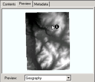
You can use the Information tool (above) to click on a pixel. It
should show you the coordinate of that pixel and the elevation. This
elevation is meaningless, of courses, unless you know the units and
the datum. Make sure that the spatial coordinate system is defined
in the file by checking “properties”.
Import the XML Metadata that you downloaded from the CUGIR site
into the dataset. You notice that the units of elevation are in
meters, and the resolution of the data is given as "1" with
a unit of decimeters. This means that elevations are represented with
a precision of 0.1 m. This does not mean that the DEM is accurate to
within one decimeter, however. To obtain more information about the
accuracy of the data, scroll down to "Spatial Data Quality".
Green text such as these can be expanded to provide more information
about the data. Under this category, you will see headings for
horizontal and vertical accuracy. These metadata indicate that the
data are accurate with 3 m horizontally, and 6 to 8 meters
vertically. This is important to know when you actually start to use
these data. It establishes "error bars" on the spatial
data.
If you read more about this DEM you will find that it was created
by digitizing contoured topopgraphic maps. This means that the DEM is
no more accurate than the original 1:24,000 scale quad from which it
was created. This quad is represented in the DRG file as well.
Repeat this process for the West Valley quad DEM, including the
metadata.
Go to Page 3